Exploring NASAs Top Solar Flares
- 30 minsPart 1: Data Scrapping and Preparation
Step 1: Scraping my competitor’s data
First, install some packages
install.packages("rvest")
install.packages("tibble") # a better way to print data frameslibrary(rvest) # for html parsing
library(dplyr) # for data manipulation
library(tidyr) # for TODO
library(ggplot2)
library(readr)
# the url of the page we scrape from
space_weather <- read_html("https://www.spaceweatherlive.com/en/solar-activity/top-50-solar-flares")
# useful rvest tutorial: https://www.r-bloggers.com/using-rvest-to-scrape-an-html-table/
rank_tables <- space_weather %>%
html_node(xpath = "/html/body/div[3]/div/div/div[1]/table") %>%
html_table() %>%
`colnames<-`(c("rank",
"x_classification",
"date",
"region",
"start_time",
"maximum_time",
"end_time",
"movie"))
# make rank_table a tibble for better printing
rank_tables <- tbl_df(rank_tables)
#take a look...
rank_tables## # A tibble: 50 × 8
## rank x_classification date region start_time maximum_time
## <int> <chr> <chr> <chr> <chr> <chr>
## 1 1 X28.0 2003/11/04 0486 19:29 19:53
## 2 2 X20 2001/04/02 9393 21:32 21:51
## 3 3 X17.2 2003/10/28 0486 09:51 11:10
## 4 4 X17.0 2005/09/07 0808 17:17 17:40
## 5 5 X14.4 2001/04/15 9415 13:19 13:50
## 6 6 X10.0 2003/10/29 0486 20:37 20:49
## 7 7 X9.4 1997/11/06 - 11:49 11:55
## 8 8 X9.0 2006/12/05 0930 10:18 10:35
## 9 9 X8.3 2003/11/02 0486 17:03 17:25
## 10 10 X7.1 2005/01/20 0720 06:36 07:01
## # ... with 40 more rows, and 2 more variables: end_time <chr>, movie <chr>Step 2: Tidy the top 50 solar flare data
Your next step is to make sure this table is usable using the dplyr and tidyr packages:
- Drop the last column of the table, since we are not going to use it moving forward.
rank_tables <- rank_tables %>% select(-movie)- Use the tidyr::unite package to combine the date and each of the three time columns into three datetime columns. You will see why this is useful later on.
# unite the date with each of the three times, seperate by space, do not remove input columns
rank_tables <- rank_tables %>% unite("start_datetime", date, start_time, sep = " ", remove=FALSE)
rank_tables <- rank_tables %>% unite("max_datetime", date, maximum_time, sep = " ", remove=FALSE)
rank_tables <- rank_tables %>% unite("end_datetime", date, end_time, sep = " ", remove=FALSE)

# remove the date, start_time, maximum_time, end_time, now that we don't need them
rank_tables <- rank_tables %>% select(-date, -start_time, -maximum_time, -end_time)- Set regions coded as - as missing (NA). You can use stringr::str_detect here.
rank_tables <- rank_tables %>%
mutate(region = ifelse(stringr::str_detect("-", region), NA, region))- Use the
readr::type_convert` function to convert columns containing datetimes into actual datetime objects.
rank_tables <- rank_tables %>% readr::type_convert(col_types = cols(
  start_datetime = col_datetime(format="%Y/%m/%d %H:%M"),
  end_datetime = col_datetime(format="%Y/%m/%d %H:%M"),
  max_datetime = col_datetime(format="%Y/%m/%d %H:%M")
))
The result of this step should be a data frame with the first few rows as:
rank_tables## # A tibble: 50 × 6
## rank x_classification start_datetime max_datetime
## <int> <chr> <dttm> <dttm>
## 1 1 X28.0 2003-11-04 19:29:00 2003-11-04 19:53:00
## 2 2 X20 2001-04-02 21:32:00 2001-04-02 21:51:00
## 3 3 X17.2 2003-10-28 09:51:00 2003-10-28 11:10:00
## 4 4 X17.0 2005-09-07 17:17:00 2005-09-07 17:40:00
## 5 5 X14.4 2001-04-15 13:19:00 2001-04-15 13:50:00
## 6 6 X10.0 2003-10-29 20:37:00 2003-10-29 20:49:00
## 7 7 X9.4 1997-11-06 11:49:00 1997-11-06 11:55:00
## 8 8 X9.0 2006-12-05 10:18:00 2006-12-05 10:35:00
## 9 9 X8.3 2003-11-02 17:03:00 2003-11-02 17:25:00
## 10 10 X7.1 2005-01-20 06:36:00 2005-01-20 07:01:00
## # ... with 40 more rows, and 2 more variables: end_datetime <dttm>,
## # region <chr>Step 3. Scrape the NASA data (15 pts)
waves <- read_html("http://www.hcbravo.org/IntroDataSci/misc/waves_type2.html")

text <- waves %>% html_node(xpath = "/html/body/pre") %>%
  html_text()

# split the text by line and restore it as a vector
text <- stringr::str_split(text, "\n")

# save the long string as a data frame
wind_tab <- tbl_df(data.frame(text))

# rename the single column of the data frame to 'first'
names(wind_tab)[1] <- "first"

# only select the lines of text that start with a date (i.e. the filter for the data we want)
wind_tab <- wind_tab %>% filter(first = stringr::str_detect(first, "\\d{4}\\/\\d{2}\\/\\d{2}"))
## Error: filter() takes unnamed arguments. Do you need `==`?# create a column names vector (we ignore the link and the notes columns)
col_names <- c("start_date",
"start_time",
"end_date",
"end_time",
"start_frequency",
"end_frequency",
"flare_location",
"flare_region",
"flare_classification",
"cme_date",
"cme_time",
"cme_angle",
"cme_width",
"cme_speed")
# seperate column by spaces, ignore the warning about too many values: this happens because we are
# not seperating past the cme_speed column and ignoring it (and also the notes column for some of
# the entities)
wind_tab <- wind_tab %>% tidyr::separate(col = "first", into = col_names, sep = "\\s+")## Warning: Too many values at 483 locations: 11, 13, 14, 15, 16, 17, 18, 19,
## 20, 21, 22, 23, 24, 25, 26, 27, 28, 29, 30, 31, ...## Warning: Too few values at 13 locations: 1, 2, 4, 5, 6, 7, 8, 9, 10, 12,
## 495, 496, 497# take a look...
wind_tab## # A tibble: 497 × 14
## start_date
## * <chr>
## 1
## 2 NOTE:
## 3 but
## 4 frequencies
## 5 observations
## 6
## 7 ===========================================================================
## 8
## 9 ----------------------------------------
## 10 Start
## # ... with 487 more rows, and 13 more variables: start_time <chr>,
## # end_date <chr>, end_time <chr>, start_frequency <chr>,
## # end_frequency <chr>, flare_location <chr>, flare_region <chr>,
## # flare_classification <chr>, cme_date <chr>, cme_time <chr>,
## # cme_angle <chr>, cme_width <chr>, cme_speed <chr>Step 4:Tidy the NASA the table (15 pts)
Now, we tidy up the NASA table. Here we will code missing observations properly, recode columns that correspond to more than one piece of information, treat dates and times appropriately, and finally convert each column to the appropriate data type.
- Recode any missing entries as NA. Refer to the data description in to see how missing entries are encoded in each column.
# Frequency
# replace start_frequency
wind_tab <- wind_tab %>%
mutate(start_frequency = ifelse((start_frequency == "????"), NA, start_frequency))
# replace end_frequency
wind_tab <- wind_tab %>%
mutate(end_frequency = ifelse((end_frequency == "????"), NA, end_frequency))
# Flare
# replace source region location (flare_location)
wind_tab <- wind_tab %>%
mutate(flare_location = ifelse((flare_location == "------"), NA, flare_location))
# replace active region location (flare_region)
wind_tab <- wind_tab %>%
mutate(flare_region = ifelse((flare_region == "-----"), NA, flare_region))
# replace flare impotence (flare_classification)
wind_tab <- wind_tab %>%
mutate(flare_classification = ifelse((flare_classification == "----"), NA, flare_classification))
# CME Parameters
# replace cme_date
wind_tab <- wind_tab %>%
mutate(cme_date = ifelse((cme_date == "--/--"), NA, cme_date))
# replace cme_time
wind_tab <- wind_tab %>%
mutate(cme_time = ifelse((cme_time == "--:--"), NA, cme_time))
# replace cme_angle (cme CPA)
wind_tab <- wind_tab %>%
mutate(cme_angle = ifelse((cme_angle == "----"), NA, cme_angle))
# replace cme_width (need to replace both 3-dashes and 4-dashes)
wind_tab <- wind_tab %>%
mutate(cme_width = ifelse((cme_width == "---"), NA, cme_width))
wind_tab <- wind_tab %>%
mutate(cme_width = ifelse((cme_width == "----"), NA, cme_width))
# replace cme_speed
wind_tab <- wind_tab %>%
mutate(cme_speed = ifelse((cme_speed == "----"), NA, cme_speed))- The CPA column (cme angle) contains angles in degrees for most rows, except for halo flares, which are coded as Halo. Create a new column that indicates if a row corresponds to a halo flare or not, and then replace Halo entries in the cme_angle column as NA.
wind_tab <- wind_tab %>% mutate(cme_halo = ((cme_angle) == "Halo"))
wind_tab <- wind_tab %>% mutate(cme_angle = ifelse((cme_angle == "Halo"), NA, cme_angle))- The width column indicates if the given value is a lower bound. Create a new column that indicates if width is given as a lower bound, and remove any non-numeric part of the width column.
# make logical vector (attribute) cme_width_lb
wind_tab <- wind_tab %>% mutate(cme_width_lb = stringr::str_detect(cme_width, ">\\d+"))
# remove the '>' symbol
wind_tab <- wind_tab %>% mutate(cme_width = sub(">","",cme_width))- Combine date and time columns for start, end and cme so they can be encoded as datetime objects.
# unite the date with each of the three times, seperate by space, do not remove input columns
wind_tab <- wind_tab %>% unite("start_datetime", start_date, start_time, sep = " ", remove=FALSE)
# extract start year for end_datetime and cme_datetime
wind_tab <- wind_tab %>%
separate("start_date", into = "start_dateyear", sep = "/", remove=FALSE, extra = "drop")
wind_tab <- wind_tab %>%
unite("end_datetime", start_dateyear, end_date, end_time, sep = " ", remove=FALSE)
wind_tab <- wind_tab %>%
unite("cme_datetime", start_dateyear, cme_date, cme_time, sep = " ", remove=FALSE)
# remove the date, start_time, maximum_time, end_time, now that we don't need them
wind_tab <- wind_tab %>%
select(-start_date, -start_time, -end_date, -end_time, -cme_time, -cme_date,-start_dateyear)- Use the readr::type_convert function to convert columns to appropriate types.
# convert the <chr> columns to <datetime>
wind_tab <- wind_tab %>% readr::type_convert(col_types = cols(
start_datetime = col_datetime(format="%Y/%m/%d %H:%M"),
end_datetime = col_datetime(format="%Y %m/%d %H:%M"),
cme_datetime = col_datetime(format="%Y %m/%d %H:%M")
))
# take a look...
wind_tab
## # A tibble: 497 × 13
## start_datetime end_datetime cme_datetime start_frequency end_frequency
## * <dttm> <dttm> <dttm> <chr> <chr>
## 1 <NA> <NA> <NA> <NA> <NA>
## 2 <NA> <NA> <NA> type II
## 3 <NA> <NA> <NA> on Oct
## 4 <NA> <NA> <NA> determined using
## 5 <NA> <NA> <NA> <NA> <NA>
## 6 <NA> <NA> <NA> <NA> <NA>
## 7 <NA> <NA> <NA> <NA> <NA>
## 8 <NA> <NA> <NA> Flare CME
## 9 <NA> <NA> <NA> <NA> <NA>
## 10 <NA> <NA> <NA> NOAA Imp
## # ... with 487 more rows, and 8 more variables: flare_location <chr>,
## # flare_region <chr>, flare_classification <chr>, cme_angle <chr>,
## # cme_width <chr>, cme_speed <chr>, cme_halo <lgl>, cme_width_lb <lgl>Part 2: Analysis
Now that you have data from both sites, let’s start some analysis.
Question 1: Replication (10 pts)
Can you replicate the top 50 solar flare table in SpaceWeatherLive.com exactly using the data obtained from NASA? That is, if you get the top 50 solar flares from the NASA table based on their classification (e.g., X28 is the highest), do you get data for the same solar flare events?
Include code used to get the top 50 solar flares from the NASA table (be careful when ordering by classification, using tidyr::separate here is useful). Write a sentence or two discussing how well you can replicate the SpaceWeatherLive data from the NASA data.
# seperate flare_classification into main classification and sub classification
tmp <- wind_tab  %>% separate("flare_classification", into = c("main_classification",
                                                               "sub_classification"),
                              sep = "\\.", remove=FALSE)

# seperate main classification into its letter and number
tmp <- tmp  %>%
  separate("main_classification", into = c("main_letter_class",
                                           "main_num_class"),
           sep = 1,
           remove=FALSE)

# convert the classification <chr> to <int>
tmp <- tmp %>% readr::type_convert(col_types = cols(
  main_num_class = col_integer(),
  sub_classification = col_integer()
))

# order the classification by letter and number
top_class <- tmp %>%
  arrange(desc(main_letter_class), desc(main_num_class), desc(sub_classification)) %>%
    select(flare_classification)

# display the top 50 classifications side by side
data.frame(rank_tables$rank, top_class[1:50,], rank_tables$x_classification)
## rank_tables.rank flare_classification rank_tables.x_classification
## 1 1 X28. X28.0
## 2 2 X20. X20
## 3 3 X17. X17.2
## 4 4 X14. X17.0
## 5 5 X10. X14.4
## 6 6 X9.4 X10.0
## 7 7 X9.0 X9.4
## 8 8 X8.3 X9.0
## 9 9 X7.1 X8.3
## 10 10 X6.9 X7.1
## 11 11 X6.5 X6.9
## 12 12 X6.2 X6.5
## 13 13 X5.7 X6.2
## 14 14 X5.6 X6.2
## 15 15 X5.4 X5.7
## 16 16 X5.3 X5.6
## 17 17 X4.9 X5.4
## 18 18 X4.8 X5.4
## 19 19 X4.0 X5.4
## 20 20 X3.9 X5.3
## 21 21 X3.8 X4.9
## 22 22 X3.6 X4.9
## 23 23 X3.4 X4.8
## 24 24 X3.4 X4.0
## 25 25 X3.3 X3.9
## 26 26 X3.2 X3.9
## 27 27 X3.1 X3.8
## 28 28 X2.8 X3.7
## 29 29 X2.7 X3.6
## 30 30 X2.7 X3.6
## 31 31 X2.6 X3.6
## 32 32 X2.6 X3.4
## 33 33 X2.6 X3.4
## 34 34 X2.5 X3.3
## 35 35 X2.3 X3.3
## 36 36 X2.3 X3.3
## 37 37 X2.3 X3.2
## 38 38 X2.2 X3.1
## 39 39 X2.1 X3.1
## 40 40 X2.1 X3.0
## 41 41 X2.1 X2.8
## 42 42 X2.1 X2.8
## 43 43 X2.0 X2.8
## 44 44 X2.0 X2.7
## 45 45 X2.0 X2.7
## 46 46 X2.0 X2.7
## 47 47 X1.9 X2.6
## 48 48 X1.8 X2.6
## 49 49 X1.8 X2.6
## 50 50 X1.8 X2.5As you can see, we can match many of the data points by comparing the classifications once we order them. Our replication effort is okay.
Question 2: Integration (15 pts)
Below is the code I use to join the two tables, I explain my reasoning about it after this code block.
# seperate flare_classification into main classification and sub classification
wind_w_class <- wind_tab  %>%
  separate("flare_classification", into = c("main_classification",
                                            "sub_classification"),
           sep = "\\.", remove=FALSE)

# seperate x_classification into main classification and sub classification
rank_w_class <- rank_tables %>%
  separate("x_classification", into = c("main_classification",
                                        "sub_classification"),
           sep = "\\.", remove=FALSE)

# seperate date and time of wind_w_class
wind_w_class <- wind_w_class  %>%
  separate("start_datetime", into = c("startdate", "starttime"), sep = " ", remove=FALSE)

# seperate date and time of rank_w_class
rank_w_class <- rank_w_class  %>%
  separate("start_datetime", into = c("startdate", "starttime"), sep = " ", remove=FALSE)
I tried to join the table of the top 50 with our large NASA solar flare table based off of which entities shared the same main classification and also occured on the same date. This is because there are descrepencies between how the two data sources classified a solar flare (for example, some data points in my wind_tab don’t have subclassifications while those in the rank table do).
# the third rank solar flare (from rank_tables) has a classification of 'X17.2' while on the
#wind_tab, the same corresponding classification is a 'X17.', notice the missing '.2'

# has no sub_classification (notice nothing prints under the sub_classification column)
wind_w_class %>%
  filter(stringr::str_detect(main_classification, "X17")) %>%
    select(start_datetime, flare_classification, main_classification, sub_classification)
## # A tibble: 1 × 4
## start_datetime flare_classification main_classification
## <dttm> <chr> <chr>
## 1 2003-10-28 11:10:00 X17. X17
## # ... with 1 more variables: sub_classification <chr># HAS a sub_classification
rank_w_class %>%
filter(stringr::str_detect(main_classification, "X17")) %>%
select(start_datetime, main_classification, sub_classification, rank)## # A tibble: 2 × 4
## start_datetime main_classification sub_classification rank
## <dttm> <chr> <chr> <int>
## 1 2003-10-28 09:51:00 X17 2 3
## 2 2005-09-07 17:17:00 X17 0 4This is a good example because it tells us that the main classification is not enough alone to join these two tables. The second table that was printed has two different ranks (3 and 4, respectively) for the same main classification. The only difference (apart from the sub_classification) that we can use to compare with our NASA table is the start datetime. But as you can see, the two different tables have a matching date but not a matching time. Therefore we split the datetime into a date and a time and only match by the date.
# from the code above
# seperate date and time of wind_w_class
wind_w_class <- wind_w_class  %>%
  separate("start_datetime", into = c("startdate", "starttime"), sep = " ", remove=FALSE)

# seperate date and time of rank_w_class
rank_w_class <- rank_w_class %>%
  separate("start_datetime", into = c("startdate", "starttime"), sep = " ", remove=FALSE)
After doing this, we have enough information to join/merge/integrate our two tables. We however will miss out on some data. For example, we cannot merge the 4th ranked solar flare (see above) because it does not correspond to any solar flare that occured on the same date and have the same classification. After merging, we can successfully match 34 out of the 50 data points from the top 50.
We add the ranks to our larger NASA dataset below
# only keep primary key (classification and startdate) from the rank table
rank_w_class <- rank_w_class %>%
  select(rank, main_classification, startdate)

# left join the ranks to the large nasa table (i.e. wind_w_class)
wind_w_class <- wind_w_class %>%
  left_join(rank_w_class, by = c("main_classification", "startdate"))

# remove the splited columns we created
wind_w_class <- wind_w_class %>%
  select(-main_classification, -sub_classification, -startdate, -starttime)

# set our original wind_tab to this new one that includes rank information
wind_tab <- wind_w_class

# take a look...
wind_tab
## # A tibble: 497 × 14
## start_datetime end_datetime cme_datetime start_frequency end_frequency
## <dttm> <dttm> <dttm> <chr> <chr>
## 1 <NA> <NA> <NA> <NA> <NA>
## 2 <NA> <NA> <NA> type II
## 3 <NA> <NA> <NA> on Oct
## 4 <NA> <NA> <NA> determined using
## 5 <NA> <NA> <NA> <NA> <NA>
## 6 <NA> <NA> <NA> <NA> <NA>
## 7 <NA> <NA> <NA> <NA> <NA>
## 8 <NA> <NA> <NA> Flare CME
## 9 <NA> <NA> <NA> <NA> <NA>
## 10 <NA> <NA> <NA> NOAA Imp
## # ... with 487 more rows, and 9 more variables: flare_location <chr>,
## # flare_region <chr>, flare_classification <chr>, cme_angle <chr>,
## # cme_width <chr>, cme_speed <chr>, cme_halo <lgl>, cme_width_lb <lgl>,
## # rank <int># and also w/rank
wind_tab %>%
select(start_datetime, flare_classification, rank)## # A tibble: 497 × 3
## start_datetime flare_classification rank
## <dttm> <chr> <int>
## 1 <NA> <NA> NA
## 2 <NA> by NA
## 3 <NA> start NA
## 4 <NA> and NA
## 5 <NA> <NA> NA
## 6 <NA> <NA> NA
## 7 <NA> <NA> NA
## 8 <NA> <NA> NA
## 9 <NA> <NA> NA
## 10 <NA> CPA NA
## # ... with 487 more rowsTada!
Question 3: Analysis (10 pts)
Prepare one plot that shows the top 50 solar flares in context with all data available in the NASA dataset. Lets do some data visualizations!
# cme_speed changing over the years
wind_tab %>%
  mutate(month = (format(start_datetime, "%m"))) %>%
    group_by("month") %>%
      ggplot(aes(x=start_datetime, y=cme_speed)) +
        geom_smooth() +
          xlab("Date") +
          ylab("CME Speed")
## `geom_smooth()` using method = 'loess'## Warning: Removed 15 rows containing non-finite values (stat_smooth).## Warning in simpleLoess(y, x, w, span, degree = degree, parametric =
## parametric, : span too small. fewer data values than degrees of freedom.## Warning in simpleLoess(y, x, w, span, degree = degree, parametric =
## parametric, : at 9.2983e+08## Warning in simpleLoess(y, x, w, span, degree = degree, parametric =
## parametric, : radius 8.4586e+10## Warning in simpleLoess(y, x, w, span, degree = degree, parametric =
## parametric, : all data on boundary of neighborhood. make span bigger## Warning in simpleLoess(y, x, w, span, degree = degree, parametric =
## parametric, : pseudoinverse used at 9.2983e+08## Warning in simpleLoess(y, x, w, span, degree = degree, parametric =
## parametric, : neighborhood radius 2.9084e+05## Warning in simpleLoess(y, x, w, span, degree = degree, parametric =
## parametric, : reciprocal condition number 1## Warning in simpleLoess(y, x, w, span, degree = degree, parametric =
## parametric, : at 9.8858e+08## Warning in simpleLoess(y, x, w, span, degree = degree, parametric =
## parametric, : radius 8.4586e+10## Warning in simpleLoess(y, x, w, span, degree = degree, parametric =
## parametric, : all data on boundary of neighborhood. make span bigger## Warning in simpleLoess(y, x, w, span, degree = degree, parametric =
## parametric, : There are other near singularities as well. 8.4586e+10## Warning in simpleLoess(y, x, w, span, degree = degree, parametric =
## parametric, : zero-width neighborhood. make span bigger## Warning in simpleLoess(y, x, w, span, degree = degree, parametric =
## parametric, : zero-width neighborhood. make span bigger## Warning: Computation failed in `stat_smooth()`:
## NA/NaN/Inf in foreign function call (arg 5)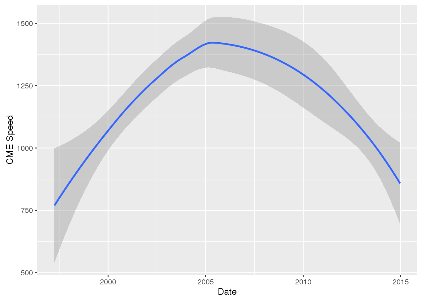
# cme_speed vs cme_width of the top 50
wind_tab %>% filter(!is.na(rank)) %>%
  ggplot(aes(x=cme_speed, y =cme_width, label = rank))  +
    geom_text() +
    geom_smooth()
## `geom_smooth()` using method = 'loess'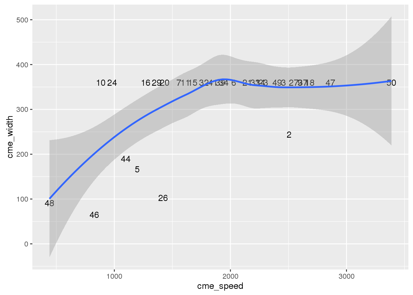
Do strong flares cluster in time? Plot the number of flares per month over time, add a graphical element to indicate (e.g., text or points) to indicate the number of strong flares (in the top 50) to see if they cluster.
# plot a bar graph of the number of flares per month and cluster the strong (top 50) from the weak
 wind_tab %>%
  mutate(month = (format(start_datetime, "%m")), top_50 = !is.na(rank)) %>%
    group_by(month,is.na(rank)) %>%
      ggplot(aes(x = month,fill=top_50)) + geom_bar()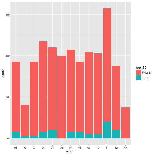

Yusuf Ameri
Learning Since 1997